Create distributions3 Object

A single class and corresponding methods encompassing all bamlss.family distributions (from the bamlss package) using the workflow from the distributions3 package.

BAMLSS(family, ...)

Arguments

family

object. BAMLSS family specifications recognized by bamlss.family, including family.bamlss objects, family-generating functions (e.g., gaussian_bamlss), or characters with family names (e.g., "gaussian" or "binomial").

...

further arguments passed as parameters to the BAMLSS family. Can be scalars or vectors.

Value

A BAMLSS distribution object.

Details

The constructor function BAMLSS sets up a distribution object, representing a distribution from the BAMLSS (Bayesian additive model of location, scale, and shape) framework by the corresponding parameters plus a family attribute, e.g., gaussian_bamlss for the normal distribution or binomial_bamlss for the binomial distribution. The parameters employed by the family vary across the families but typically capture different distributional properties (like location, scale, shape, etc.).

All parameters can also be vectors, so that it is possible to define a vector of BAMLSS distributions from the same family with potentially different parameters. All parameters need to have the same length or must be scalars (i.e., of length 1) which are then recycled to the length of the other parameters.

For the BAMLSS distribution objects there is a wide range of standard methods available to the generics provided in the distributions3 package: pdf and log_pdf for the (log-)density (PDF), cdf for the probability from the cumulative distribution function (CDF), quantile for quantiles, random for simulating random variables, and support for the support interval (minimum and maximum). Internally, these methods rely on the usual d/p/q/r functions provided in bamlss, see the manual pages of the individual families. The methods is_discrete and is_continuous can be used to query whether the distributions are discrete on the entire support or continuous on the entire support, respectively.

See the examples below for an illustration of the workflow for the class and methods.

See also

bamlss.family

Examples

 if(!requireNamespace("bamlss")) {
  if(interactive() || is.na(Sys.getenv("_R_CHECK_PACKAGE_NAME_", NA))) {
    stop("not all packages required for the example are installed")
  } else q() }

## package and random seed
library("distributions3")
set.seed(6020)

## three Weibull distributions
X <- BAMLSS("weibull", lambda = c(1, 1, 2), alpha = c(1, 2, 2))
X
#> [1] "BAMLSS weibull distribution (lambda = 1, alpha = 1)"
#> [2] "BAMLSS weibull distribution (lambda = 1, alpha = 2)"
#> [3] "BAMLSS weibull distribution (lambda = 2, alpha = 2)"

## moments (FIXME: mean and variance not provided by weibull_bamlss)
## mean(X)
## variance(X)

## support interval (minimum and maximum)
support(X)
#>      min max
#> [1,]   0 Inf
#> [2,]   0 Inf
#> [3,]   0 Inf
is_discrete(X)
#> [1] FALSE FALSE FALSE
is_continuous(X)
#> [1] TRUE TRUE TRUE

## simulate random variables
random(X, 5)
#>           r_1       r_2       r_3      r_4      r_5
#> [1,] 1.004812 0.3993868 1.3084904 0.741085 3.209012
#> [2,] 1.023982 0.5593371 0.5440658 1.046042 2.244104
#> [3,] 1.254624 2.8848168 3.0103388 2.166692 2.572731

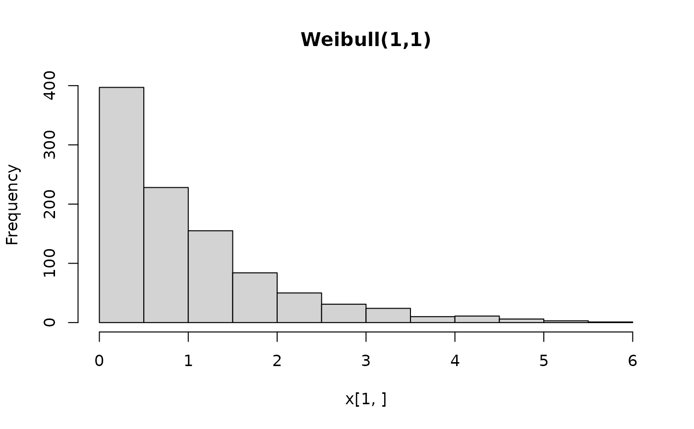
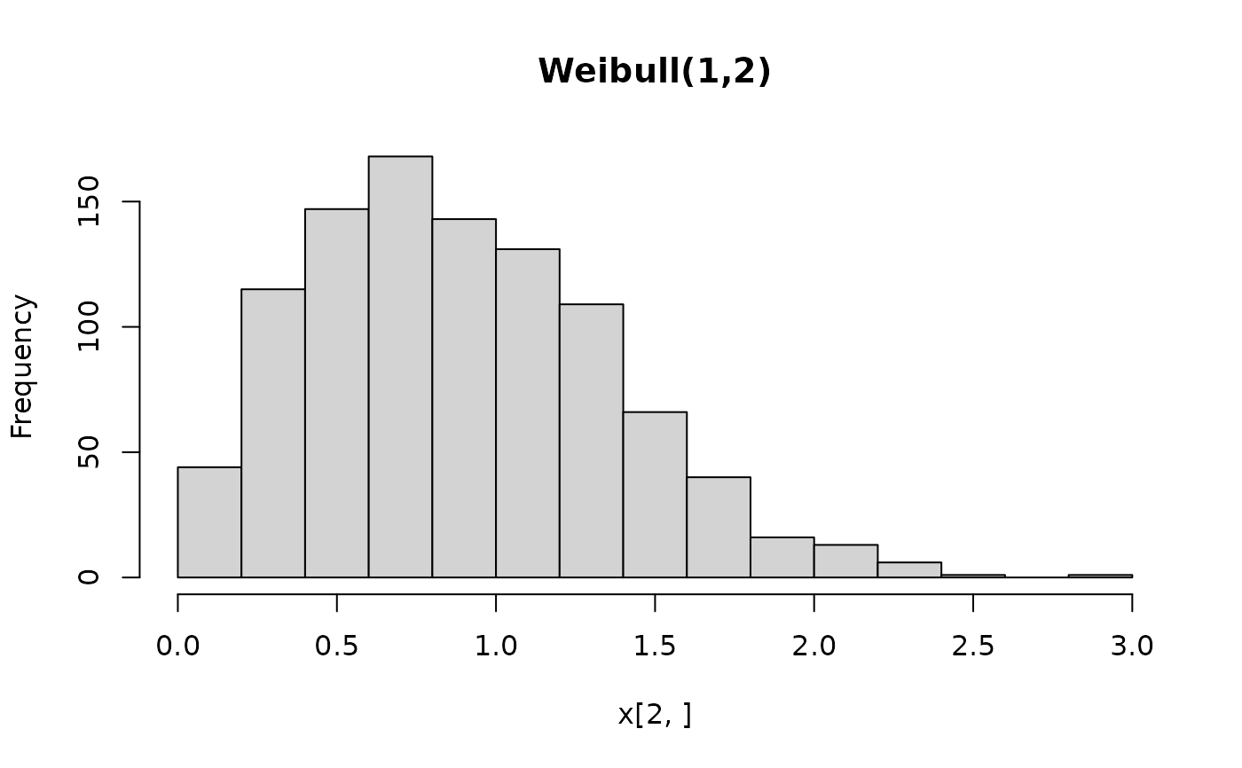
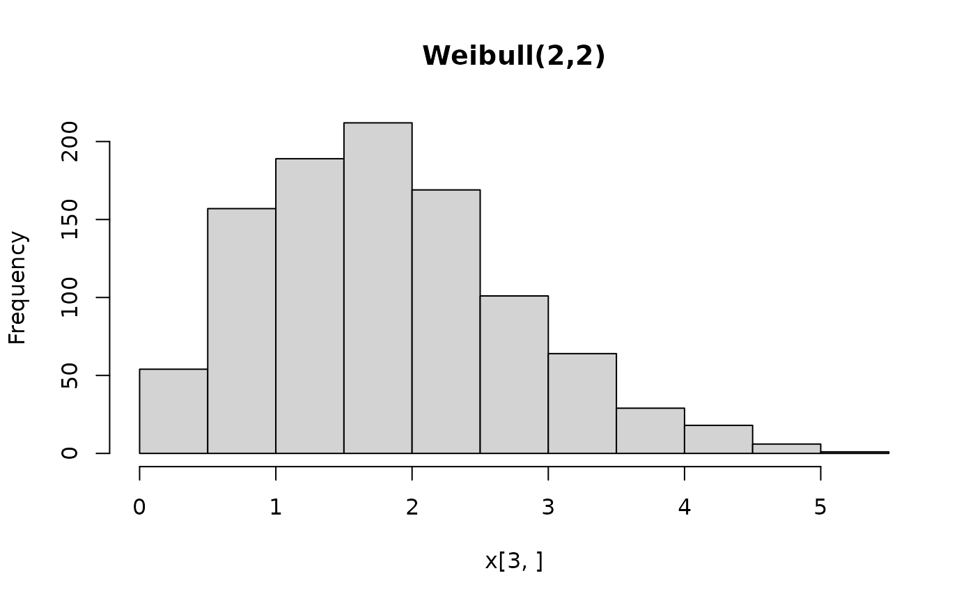
## histograms of 1,000 simulated observations
x <- random(X, 1000)
hist(x[1, ], main = "Weibull(1,1)")

hist(x[2, ], main = "Weibull(1,2)")

hist(x[3, ], main = "Weibull(2,2)")


## probability density function (PDF) and log-density (or log-likelihood)
x <- c(2, 2, 1)
pdf(X, x)
#> [1] 0.13533528 0.07326256 0.38940039
pdf(X, x, log = TRUE)
#> [1] -2.0000000 -2.6137056 -0.9431472
log_pdf(X, x)
#> [1] -2.0000000 -2.6137056 -0.9431472

## cumulative distribution function (CDF)
cdf(X, x)
#> [1] 0.8646647 0.9816844 0.2211992

## quantiles
quantile(X, 0.5)
#> [1] 0.6931472 0.8325546 1.6651092

## cdf() and quantile() are inverses
cdf(X, quantile(X, 0.5))
#> [1] 0.5 0.5 0.5
quantile(X, cdf(X, 1))
#> [1] 1 1 1

## all methods above can either be applied elementwise or for
## all combinations of X and x, if length(X) = length(x),
## also the result can be assured to be a matrix via drop = FALSE
p <- c(0.05, 0.5, 0.95)
quantile(X, p, elementwise = FALSE)
#>          q_0.05     q_0.5   q_0.95
#> [1,] 0.05129329 0.6931472 2.995732
#> [2,] 0.22648023 0.8325546 1.730818
#> [3,] 0.45296046 1.6651092 3.461637
quantile(X, p, elementwise = TRUE)
#> [1] 0.05129329 0.83255461 3.46163677
quantile(X, p, elementwise = TRUE, drop = FALSE)
#>        quantile
#> [1,] 0.05129329
#> [2,] 0.83255461
#> [3,] 3.46163677

## compare theoretical and empirical mean from 1,000 simulated observations
## (FIXME: mean not provided by weibull_bamlss)
## cbind(
##   "theoretical" = mean(X),
##   "empirical" = rowMeans(random(X, 1000))
## )